Fitxer:Master equation unravelings.svg
Salta a la navegació
Salta a la cerca

Mida d'aquesta previsualització PNG del fitxer SVG: 720 × 540 píxels. Altres resolucions: 320 × 240 píxels | 640 × 480 píxels | 1.024 × 768 píxels | 1.280 × 960 píxels | 2.560 × 1.920 píxels.
Fitxer original (fitxer SVG, nominalment 720 × 540 píxels, mida del fitxer: 453 Ko)
Resum
| Descripció |
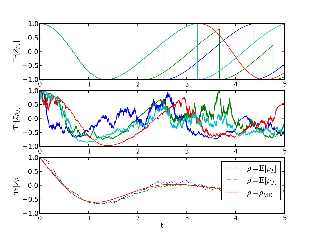
English: Plot of the evolution of the z-component of the Bloch vector of a two-level atom coupled to the electromagnetic field undergoing damped Rabi oscillations. The top plot shows the quantum trajectory for the atom for photon-counting measurements performed on the electromagnetic field, the middle plot shows the same for homodyne detection, and the bottom plot compares the previous two measurement choices (each averaged over 32 trajectories) with the unconditioned evolution given by the master equation. |
| Data | |
| Font | Treball propi |
| Autor | Azaghal of Belegost |
Source code
Source Code in python:
|
|---|
import numpy as np
import matplotlib.pyplot as plt
import sys
import random
from math import pi, cos, sin, sqrt

# Pauli matrices
X = np.matrix([[0. + 0.j, 1. + 0.j], [1. + 0.j, 0. + 0.j]])
Y = np.matrix([[0. + 0.j, 0. - 1.j], [0. + 1.j, 0. + 0.j]])
Z = np.matrix([[1. + 0.j, 0. + 0.j], [0. + 0.j, -1 + 0.j]])
Id = np.matrix([[1. + 0.j, 0. + 0.j], [0. + 0.j, 1. + 0.j]])

# Program parameters
timesteps = 1e4
final_time = 5
timestep = final_time/timesteps

# Evolution parameters
H = 1*X
g = 1
L = sqrt(g)*(X - 1.j*Y)/2

# Initial Bloch vector parameters
r = 1
theta = 0
phi = 0
initial_state = 0.5*(Id + r*(cos(theta)*Z + sin(theta)*(cos(phi)*X +
                     sin(phi)*Y)))
trials = 32

def Commutator(A, B):
    return A*B - B*A

def Diffusion(op, state):
    return op*state*op.H - 0.5*(op.H*op*state + state*op.H*op)

def Time_Deriv(hamiltonian, lindblad, state):
    return -1.j*Commutator(hamiltonian, state) + Diffusion(lindblad, state)

def Vacuum_SME_Evol(hamiltonian, lindblad, state, timestep):
    state_trace = np.trace(state*lindblad.H*lindblad)
    E_N = state_trace*timestep
    d_state = 0.5*timestep*(2*state*state_trace - lindblad.H*lindblad*state -
                            state*lindblad.H*lindblad)
    if random.uniform(0, 1) < E_N:
        d_state += lindblad*state*lindblad.H/state_trace - state
    else:
        d_state += -1.j*Commutator(hamiltonian, state)*timestep
    return d_state

def H_supop(op, state):
    return op*state + state*op.H - np.trace((op + op.H)*state)*state

def Homodyne_Vac_SME_Evol(hamiltonian, lindblad, state, timestep):
    d_state = (Diffusion(lindblad, state) -
               1.j*Commutator(hamiltonian, state))*timestep
    state_trace = np.trace(lindblad*state + state*lindblad.H)
    if random.uniform(0, 1) < (1 + sqrt(timestep)*state_trace)/2:
        d_R = sqrt(timestep)
    else:
        d_R = -sqrt(timestep)
    d_state += (d_R - state_trace*timestep)*H_supop(lindblad, state)
    return d_state

def main():
    state = initial_state
    E_z = []
    states = []
    times = np.arange(0, final_time, timestep)
# Calculate the trajectory from the master equation
    for time in times:
        states.append(state)
        E_z.append(np.trace(Z*state))
        state = state + Time_Deriv(H, L, state)*timestep

    cond_E_z = []
    hom_E_z = []
    test_var = pi
    cond_states = []
    hom_states = []
    avg_E_z = []
    avg_hom_E_z = []
# Calculate the conditional evolution for a number of trials
    for trial in range(trials):
        cond_state = initial_state
        cond_states.append([])
        cond_E_z.append([])
        hom_state = initial_state
        hom_states.append([])
        hom_E_z.append([])
        for time in times:
            cond_states[trial].append(cond_state)
            cond_E_z[trial].append(np.trace(Z*cond_state))
            cond_state = cond_state + Vacuum_SME_Evol(H, L, cond_state,
                                                      timestep)
            hom_states[trial].append(hom_state)
            hom_E_z[trial].append(np.trace(Z*hom_state))
            hom_state = hom_state + Homodyne_Vac_SME_Evol(H, L, hom_state,
                                                            timestep)

# Calculate the average behavior of the system over all trials
    for i in range(len(times)):
        sum_z = 0
        for cond_E_z_series in cond_E_z:
            sum_z += cond_E_z_series[i]
        avg_E_z.append(sum_z/len(cond_E_z))
        hom_sum_z = 0
        for hom_E_z_series in hom_E_z:
            hom_sum_z += hom_E_z_series[i]
        avg_hom_E_z.append(hom_sum_z/len(hom_E_z))

# Plot photon-counting conditional evolution for Z expectation value
    fig = plt.figure()
    ax1 = fig.add_subplot(311)
    for i in range(min(4, len(cond_E_z))):
        ax1.plot(times, cond_E_z[i])
    plt.axis([0, 5, -1, 1])
    plt.ylabel(r'$\operatorname{Tr}[Z\rho_I]$')

# Plot homodyne conditional evolution for Z expectation value
    ax2 = fig.add_subplot(312)
    for i in range(min(4, len(hom_E_z))):
        ax2.plot(times, hom_E_z[i])
    plt.axis([0, 5, -1, 1])
    plt.ylabel(r'$\operatorname{Tr}[Z\rho_J]$')

# Plot average Z behavior over conditional evolution trials against master
# equation trajectory
    ax3 = fig.add_subplot(313)
    ax3.plot(times, avg_E_z, dash_joinstyle='round', dash_capstyle='round',
        linestyle=':', label=r'$\rho=\operatorname{E}[\rho_I]$')
    ax3.plot(times, avg_hom_E_z, dash_joinstyle='round', dash_capstyle='round',
        linestyle='--', label=r'$\rho=\operatorname{E}[\rho_J]$')
    ax3.plot(times, E_z, linestyle='-', label=r'$\rho=\rho_\mathrm{ME}$')
    ax3.legend()
    plt.axis([0, 5, -1, 1])
    plt.xlabel('t')
    plt.ylabel(r'$\operatorname{Tr}[Z\rho]$')

    plt.savefig('master_eq_unravelings.svg')

if __name__ == '__main__':
    sys.exit(main())
|
Llicència
Jo, el titular dels drets d'autor d'aquest treball, el public sota la següent llicència:
Aquest fitxer està subjecte a la llicència Creative Commons Reconeixement-CompartirIgual 3.0 No adaptada.
- Sou lliure de:
- compartir – copiar, distribuir i comunicar públicament l'obra
- adaptar – fer-ne obres derivades
- Amb les condicions següents:
- reconeixement – Heu de donar la informació adequada sobre l'autor, proporcionar un enllaç a la llicència i indicar si s'han realitzat canvis. Podeu fer-ho amb qualsevol mitjà raonable, però de cap manera no suggereixi que l'autor us dóna suport o aprova l'ús que en feu.
- compartir igual – Si modifiqueu, transformeu, o creeu a partir del material, heu de distribuir les vostres contribucions sota una llicència similar o una de compatible amb l'original.
Historial del fitxer
Cliqueu una data/hora per veure el fitxer tal com era aleshores.
| Data/hora | Miniatura | Dimensions | Usuari/a | Comentari | |
|---|---|---|---|---|---|
| actual | 04:08, 10 des 2013 | | 720 × 540 (453 Ko) | wikimediacommons>Azaghal of Belegost | User created page with UploadWizard |
Ús del fitxer
La pàgina següent utilitza aquest fitxer: